When you see p = 0.003 or a 95% confidence interval of [80, 90], you might assume a certain clarity and definitiveness. A null effect is very unlikely to yield those results, right?
But be careful! Such overly simple reporting of p-values, confidence intervals, Bayes factors, or any statistical estimate could hide critical conclusion-flipping errors in the underlying methods and analyses. And particularly in applied fields, like visualization and Human-Computer Interaction (HCI), these conclusion-flipping errors may not only be common, but they may explain the majority of study results.
Here are some example scenarios where reported results may seem clear, but hidden statistical errors categorically change the conclusions. Importantly, these scenarios are not obscure, as I have found variants of these example problems in multiple papers.
False positive: Zero effect but a strong result
In this example, we’ll simulate an experiment with two conditions, A and B. They could be two interfaces whose performance you’re comparing. More details on the simulated experiment:
- Between-subject (each subject only runs in A or B, not both)
- 50 subjects
- 10 replicate trials (each subject runs in the same condition multiple times)
- Normally distributed individual differences in the baseline (SD = 1)
- Normally distributed response noise (SD = 0.1)
Here is the formula:
measure = subject_baseline + 0 * (condition == B) + trial_response_noise
Notice that the condition is multiplied by 0. The condition has no impact on the measurement. It is a true null effect. So we shouldn’t see big differences between the conditions. However, if the wrong statistical analysis is applied, a massive erroneous effect may be measured:
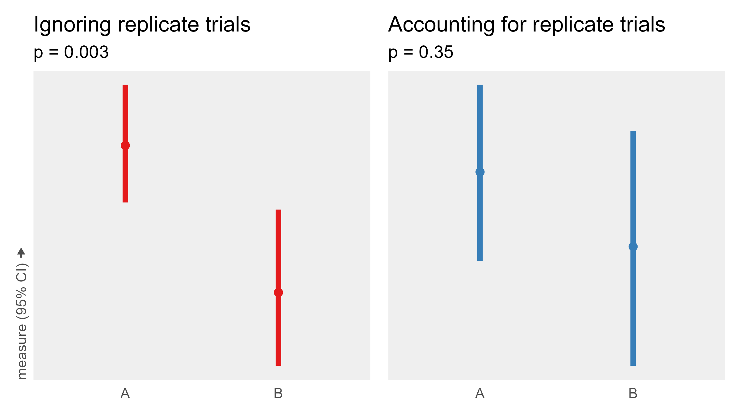
In red on the left, replicate trials are not accounted for in the analysis, yielding a large spurious difference between A and B. In blue on the right, the model reflects the experiment design, and the measured effect is indistinguishable from noise. Same data. Categorically different results. The term for this error is pseudoreplication.
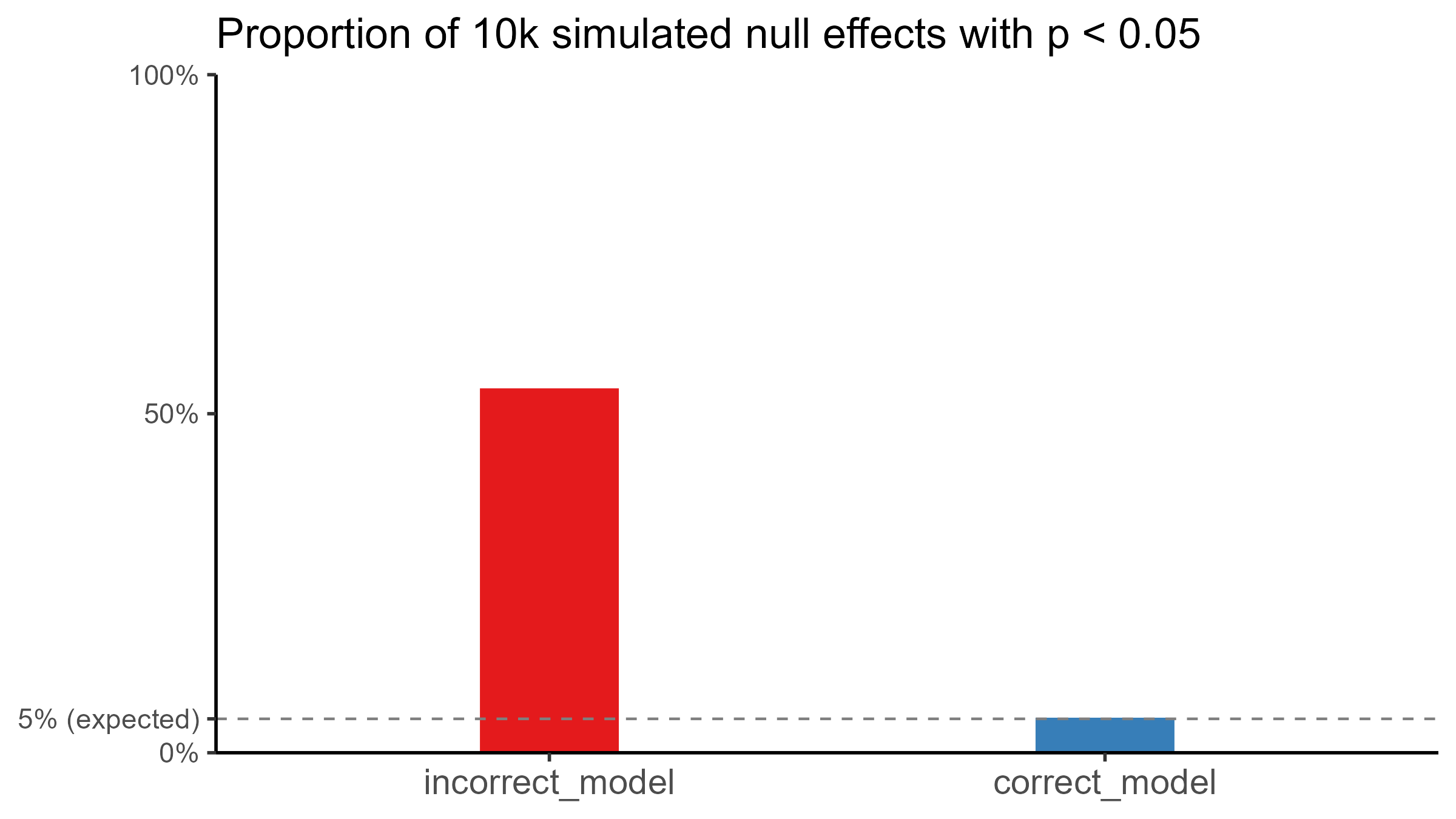
How likely a spurious effect will be found depends on the ratios of different sources of noise and the models in question. I ran 10k simulations for this specific example, and more than 50% of null effects yielded a p < 0.05, whereas the correct model had the expected 5%.
False negative: Failing to detect a very reliable effect
In this example, we’ll simulate the following experiment:
- Within-subject (each subject runs in both A and B)
- 50 subjects
- Normally distributed individual differences in the baseline (SD = 10)
- Normally distributed response noise (SD = 0.5)
Here is the formula:
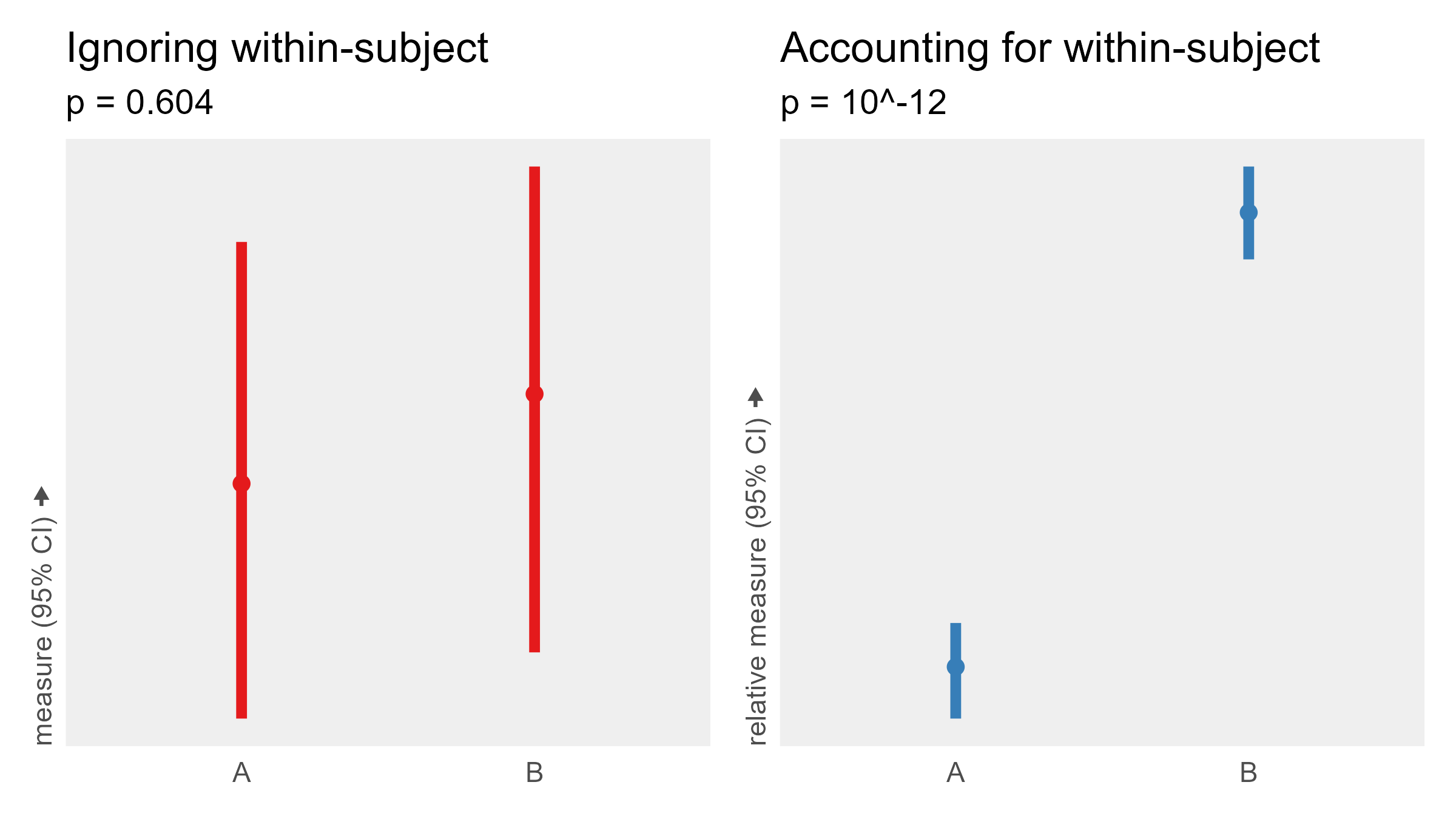
measure = subject_baseline + 1 * (condition == B) + trial_response_noise
This time, the condition variable is multiplied by one, so there is a real effect. A within-subjects experiment with 50 subjects should be able to detect that effect despite the wide range of baseline performance. However, an analysis that ignores that subjects run in both conditions fails to detect this very consistent effect.
False negative: Experiment design lacks sensitivity
This example is unlike the previous two, as it describes a methodological misstep rather than a clear-cut statistical error.
When discussing statistical power, the subject count (N) is often the only parameter brought up. But the experiment design is often critically overlooked. Many experiments leave power on the table by using between-subject designs and have no replicate trials.
We’ll simulate two different experiments with the same underlying effect.
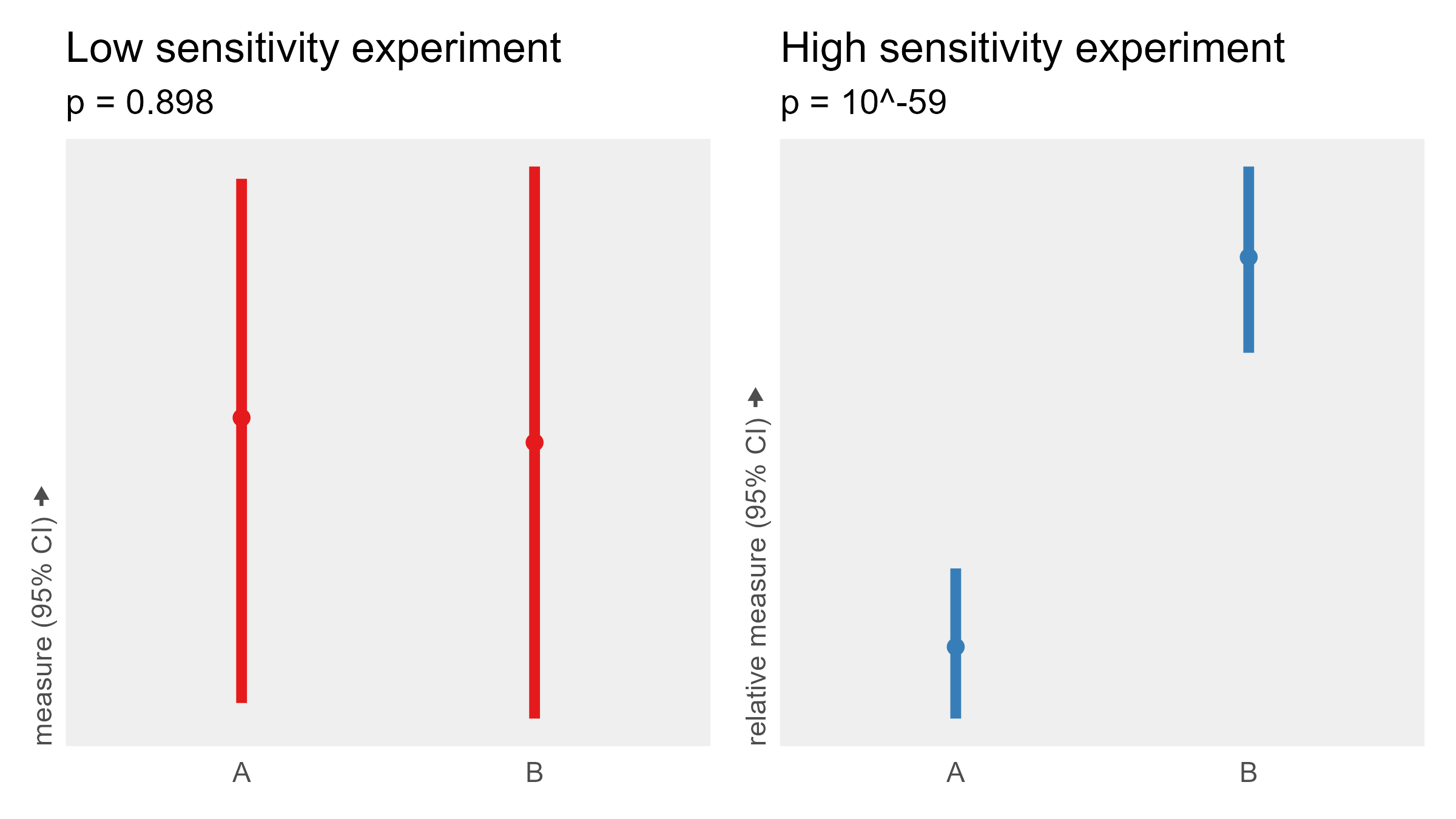
- The low-sensitivity experiment has 200 subjects who each run in one condition 1 time.
- The high-sensitivity experiment has 5 subjects who each run in both conditions 20 times.
Both experiments collect 200 total data points and use the same formula and noise levels. While the low-sensitivity experiment fails to detect an effect despite having hundreds of subjects, the high-sensitivity experiment finds the effect very clearly with only a single digit number of subjects.
I dove deeper into the impact of within-subject vs. between-subject effect sizes here and the impact of replicate trial and measurement precision here.
Red flags for spotting sketchy results
Incomplete and non-standard reporting: A p-value, an effect size, a confidence interval, or a Bayes factor is meaningless on its own. It is critical to understand how they were calculated. One of the benefits of p-values is that there are reporting standards from the APA, AMA, and other publishing bodies on how to include information like degrees of freedom and statistical estimates. Looking at the first example, there’s no way to know whether p=0.003 is correct. However, seeing F(1, 498) = 9.15, p = 0.003 for an experiment with 50 subjects and 2 conditions indicates an analysis error. 498 degrees of freedom means that the reported effect is likely inflated due to pseudoreplication. However, the degrees of freedom in F(1, 48) = 0.89, p = 0.350 match expectations from the experiment design (2-1 = 1, 25-1 + 25-1 = 48).
Unreported model: The model I used to estimate the incorrect p-value and 95% CI in the first example is measure ~ condition. However, because each subject provides multiple responses, a more appropriate model is measure ~ condition + (1|subjectID). It is surprisingly common for the model to not be reported in papers despite it often being critical to understand the validity of any statistical result.
Hidden data and code: I cannot count how many times a quick check of analysis code, data, or experiment code has revealed analysis errors that would have been undetectable with only the text. Or worse, too many papers don’t actually do what’s written in the text. It’s 2024. If code and data aren’t shared, and if a damn good reason isn’t provided, sound the bullshit alarm.
Masking naivety with modern analysis techniques: Some papers will report 95% confidence intervals or Bayesian distributions instead of p-values and claim that these approaches are immune from the various statistical concerns that p-values have. While those approaches certainly have benefits, in my experience, 95% confidence intervals are particularly prone to errors because their proponents rarely discuss that there are different ways to calculate a CI depending on the experiment design. I’ve also seen multiple authors claim that the impact of issues like multiple comparisons are not relevant if there isn’t a p-value. Most statistical concerns that apply to p-values apply regardless of technique (see Posterior Hacking from Data Colada).
Long-term solutions
There’s no shortcut to statistical education: Relying on empirical methods and statistical analyses to support the claims of one’s research without relevant education speaks volumes about one’s credibility. Unfortunately it’s very common in applied fields. Few, if any, visualization and HCI PhD curricula include even a single course in research methods. Having reviewed both cognitive science and empirical computer science research, the education difference is glaring. Many (the majority?) of empirical computer science papers have very basic statistical and methodological errors, whereas these basic errors are rare in cognitive science papers. Often, even the reviewers and editors or paper chairs have insufficient education in methods and statistics. Empirical research doesn’t stand a chance at validity, credibility, or practical utility if no one involved has the education needed to do the research correctly or spot problems should they occur.
Better reporting standards: Reporting requirements for NHST provide a lot of information to help quickly spot methodological problems. StatCheck is an example of how that standard can help detect errors. Compared to many statisticians, I’m relatively positive about NHST and p-values because the reporting standards make it easy to understand how results were calculated. But to spot a problem with a 95% CI or a Bayesian posterior distribution, I’d probably need to look at the code, which is rarely a simple process. I’d like to see approaches devised for non-NHST techniques that allow for similar quick checks.
Mandatory transparency: Open data, open analysis code, and open replication materials at the time of submission need to be the norm if we ever have chance of detecting errors. Not optional. Not encouraged. Not incentivized. Mandatory! And until such transparency is expected, science deserves any doubt and credibility concerns it gets from the public. Editors need to make it required already and enforce that requirement. Enough is enough. No consequence of requiring research transparency will ever be worse than the consequences of research validity concerns being undetectable for years or decades. Publication venues that don’t require open data, code, and materials (or an explicit reason why they can’t be shared) should be assumed to be riddled with erroneous conclusions.
Simulation and graphing code is here.
This post is part 3 of a series on statistical power and methodological errors. See also:
Simulating how replicate trial count impacts Cohen’s d effect size